This is a short note on the relationship between option pricing, Black Scholes and Defi Automated Market Makers (“AMMs”). You can read more about it in the paper – but this paper is by now 50 pages and it is worth telling this story somewhat more concisely. I will go very short on some of the issues here to please do check in the paper for details.

The relationship between AMMs and Black Scholes option pricing stems from the fact that AMMs ultimately are trading strategies. More precisely, the package AMM + arbitrageur (“the package”) is an active, self-financing trading strategy. It is well known that in a Black Scholes universe with known volatility all derivative financial instruments can be replicated with a self-financing trading strategy.

The implication of this is that whilst we may not be able to associate an easy derivative to every trading strategy, if we happen to come across a trading strategy that happens to be the replication strategy for a well-known derivative instrument (its “Delta hedge”), then for all intents and purposes this strategy is said derivative instrument.

It is a well known (and easy to prove) fact that for constant product AMM the value of their risk asset holdings always equals the value of their numeraire asset holdings. The choice of numeraire asset and risk asset here is not important, but we do need to decide one way or the other to be able to apply the Black Scholes formalism. It turns out that this trading strategy is the hedge of a well known option strategy – the square root contract.

The square root contract is a priori a European option profile – ie an option whose payoff is determined by and only by its value as a function of the spot price at some future “maturity” date $T$. If you are wondering how an indefinite trading strategy can correspond to a finite horizon European option - hang on for a second. We’ll get to that.

We have just introduced our main protagonist, the constant product AMM. Let’s now introduce the other one – the Black Scholes PDE (partial differential equation)

$$ \frac{\partial \nu}{\partial t} = -\frac{1}{2}\sigma^2\xi^2\frac{\partial^2 \nu}{\partial \xi^2} - (r-d)\xi\frac{\partial \nu}{\partial \xi} + r \nu $$

This equation establishes a relationship between the cost of hedging an option – which in an efficient market must equal its price – which is the time derivative on the left hand side. The cost is driven by the three terms on the right hand side of the equation which are, from left to right, describe

1. the bona fide option value, ie the cost caused by permanently buying high and selling low (or vice versa) depending on the “Gamma” of the position; key paramter here is the volatility $\sigma$

2. the cost of carrying the “Delta” hedge which is driven by the financing cost $r$ and the convenience or dividend yield $d$

3. the benefit of carrying the option premium over time which is again driven by the deposit rate (and financing cost) $r$

If this was somewhat short, there is a more thorough explanantion in the paper. We now define the Black Scholes operator as the spatial partial differential operator appearing on the right hand side above, ie

$$ B = -\frac{1}{2}\sigma^2\xi^2\frac{\partial^2 }{\partial \xi^2} - (r-d)\xi\frac{\partial }{\partial \xi} + r $$

It is easy to see that this operator is diagonal on the power law functions of the form $\xi^\alpha$. In other words, those functions are eigenfunctionsn satisfying the following relationship

$$ B\ \xi^\alpha = \left( -\frac{1}{2}\sigma^2 \alpha (\alpha-1) - (r-d)\alpha + r \right) \xi^\alpha $$

with the eigenvalue $\rho$ being

$$ \rho(\alpha; \sigma, r, d) = \frac{1}{2}\sigma^2\ \alpha (1-\alpha) - (r-d)\ \alpha + r $$

Note that we just solved the Black Schole equation – it turns out that on power law profiles this is much easier than on calls and puts. On the space of the $\xi^\alpha$ (which form a basis of the space of all functions) we have transformed the Black Scholes equation into a simple first order ordinary differential equation

$$ \frac{d}{dt}\ \nu_\alpha = \pm \rho\ \nu_\alpha $$

where $\rho$ is an ordinary number. That is first ODE we learn in school, and the solution to it is

$$ \nu_\alpha(t) = e^{\pm \rho t}\ \nu_\alpha(t=0) $$

The $\pm$ sign here is because we may want to get forward or backward in time (Black Scholes is solved backwards; we want to carry our strategy forwards) and the direction of time determines the sign. Now we could try to work out what the correct sign is by first principles but there is an almost 50% chance of getting it wrong along the way. Fortunately there is an easier option: we know that when going backwards in time, convex profiles always move towards the concave side (a long call options moves up and left; a long square root profile moves down and right). Moving forward in time is the opposite.

Let’s now look come back to the square root profile, ie $\alpha=\frac 1 2$. Let’s also focus on what matters – the convexity term – and ignore the delta and funding terms, ie we assume that $r=d=0$. In this case we find that

$$ \rho = \rho_{\frac 1 2} = \frac {\sigma^2} 8 $$

Let’s first do the normal Black Scholes thing, moving backwards in time, and evaluate the value today of the square root profile at time $T$. In this case we find that

$$ \nu(\xi) = e^{-\frac{\sigma^2} 8 T}\ \sqrt \xi $$

ie for $T=0$ we find the profile itself, and for longer maturities it decays over time with an exponential decay rate of $-\frac{\sigma^2} 8$. This is interesting but does not quite help us yet as we do not have a fixed maturity $T$. Instead we are moving forwards in time. This effectively means that we are not being paid an option premium upfront, but it is pay-as-you-go: we are expecting to be paid the option premium along the way.

So first let’s look at how “package” of AMM and arbitrageur – the underlying self-financing strategy – behaves in a Black Scholes world. Moving forward in time, the value of that combined position is

$$ \nu(\xi, t) = e^{\frac{\sigma^2} 8 t}\ \sqrt \xi $$

That is the pay-as-you go version of the above equation if you so want: the option premium received is proportional to $\exp(\frac{\sigma^2} 8 t)-1$. Except that it is now stochastic as it multiplies the term $\sqrt{\xi}$. We’ll come to that.

We know that the AMM does not participate in the growth at all (as we discuss in the paper the AMM does not receive any of the Gamma gains; they all go to the arbitrageur). It’s share on the value of the strategy is therefore

$$ \nu_{\mathrm{AMM}}(\xi, t) = \sqrt \xi $$

which means that the share of the arbitrageurs is

$$ \nu_{\mathrm{ARB}}(\xi, t) = \left( e^{\frac{\sigma^2} 8 t}-1\right) \ \sqrt \xi $$

Again this is stochastic. However, we can of course value it. From the equivalence between stochastic process and PDEs we know the

$$ E_{t=0}\ \left[\nu_{\mathrm{ARB}}(\xi, t=T) \right]= e^{-\frac{\sigma^2} 8 T} \left( e^{\frac{\sigma^2} 8 T}-1\right) \ \sqrt \xi_0 = \left( 1- e^{-\frac{\sigma^2} 8 T}\right) \ \sqrt \xi_0 $$

The $\xi_0$ above is the current value of $\xi$ so it is no longer stochastic. We have plotted that the above as a function of $T$ in years for a volatility of 75% (green) and 150% (orange). It is the expected percentage of value that is paid over to arbitrageurs over time, at different levels of volatility.

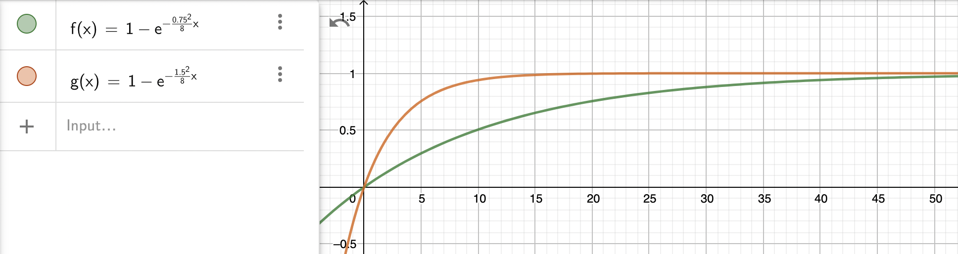
Note the term expected above: the actual outcome is stochastic, and the way the value transfer happens is that the arbitrageurs make all the gains on the Gamma, but the AMM is stuck with the divergence loss (also referred to as Impermanent Loss) in some states of the world. In other words:

the above chart shows that expected percentage of the initial investment that is lost due to divergence loss.

We need to keep in mind that this is before fees, but fees are of course another completely different kettle of fish.