Variable Weight

Key formulas

Characteristic function

$$ f(x,y) = k = x^\alpha * y^{1-\alpha} $$

The characteristic function is similar to that of a constant product AMM except that there is a weighting factor $\alpha$. For $\alpha = \frac 1 2$ we recover the standard equal weight constant product AMM.

Definition of $\eta$

$$ \eta = \frac{\alpha}{1-\alpha}\ \Rightarrow\ \alpha = \frac{\eta}{1+\eta},\ \frac{1}{1-\alpha} = 1+\eta $$

Depending on the context, the formulas with $\eta$ can be more useful than those with $\alpha$. The $\eta$ directly represents the weighting of the two assets in the pool ($\eta=1$: both assets are the same; $\eta>1$: more of the risk asset $x$).

Indifference curve ($\alpha$)

$$ y_{k,\alpha}(x) = \left( \frac k {x^\alpha} \right)^\frac 1 {1-\alpha} $$

For $\alpha = \frac 1 2$ the above formula simplifies to $k^2/x$ as expected.

Indifference curve ($\eta$)

$$ y_{k,\eta}(x) = \frac{k^{1+\eta}}{x^\eta} $$

For $\eta = 1$ the above formula simplifies to $k^2/x$ as expected.

Price response function ($\alpha$)

$$ \pi_{k,\alpha}(x) = \frac{\alpha}{1-\alpha} \left( \frac k x \right)^\frac 1 {1-\alpha} =\frac{\alpha}{1-\alpha}\ \frac {y(x)} x $$

For $\alpha = \frac 1 2$ the above formula simplifies to $(k/x)^2$. Note the $y/x$ term that is commonly seen in constant-product derived AMMs.

Price response function ($\eta$)

$$ \pi_{k,\eta}(x) = \eta \left( \frac k x \right)^{\eta+1}=\eta\ \frac {y(x)} x $$

For $\eta = 1$ the above formula simplifies to $(k/x)^2$. Note the $y/x$ term that is commonly seen in constant-product derived AMMs.

AMM portfolio value

$$ \nu(\xi) = \xi^\alpha $$

For the constant product AMM we had $\sqrt x$ in this case. We see that the value function is always a power of $\xi$. As $\alpha$ is bounded the value curves will always be similar in shape to the square root curve. For very small $\alpha$ the curve is relatively flat towards the right, and steep towards zero. For large $\alpha$ the curve gets closer to the linear curve. Note however that the apparent different in shapes is due to the choice of numeraire as the underlying AMM definition is symmetric.

Divergence loss

$$ \Lambda_\alpha(\xi) = 1-\alpha + \alpha \xi - \xi^\alpha $$

The AMM portfolio always holds $1-\alpha$ units of the numeraire asset, and has $\alpha$ units invested in the risk asset. In other words, the value ratio of risk vs numeraire asset is $\eta=\frac{\alpha}{1-\alpha}$. This is the base portfolio against which the value of AMM portfolio $\nu$ is compared for DL calculations.

Strike density function

$$ \mu(K) = -\frac{\alpha (1-\alpha)}{K^{2-\alpha}} $$

See the plots below. The strike density diverges towards zero, so complete replication with options is not possible.

Cash strike density function

$$ \mu_{\mathbf{cash}}(K) = -\frac{\alpha (1-\alpha)}{K^{1-\alpha}} $$

See the plots below. The strike density diverges towards zero, so complete replication with options is not possible.

Cash Gamma

$$ \Gamma_{\mathbf{cash}}(K) = - \alpha (1-\alpha) K^\alpha $$

See the plots below.

---

Notes

The variable weight AMM is a full range AMM, so it will never run out of assets, regardless of the price. It does allow however to see the portfolio with a different proportion of the two assets. This can be useful in a hub-and-spoke AMM design where it allows to reduce the holdings of the “hub” asset common to all pools. It also allows to create “token vending machines” that predominantly contain the token to be distributed and very little of the cash token.

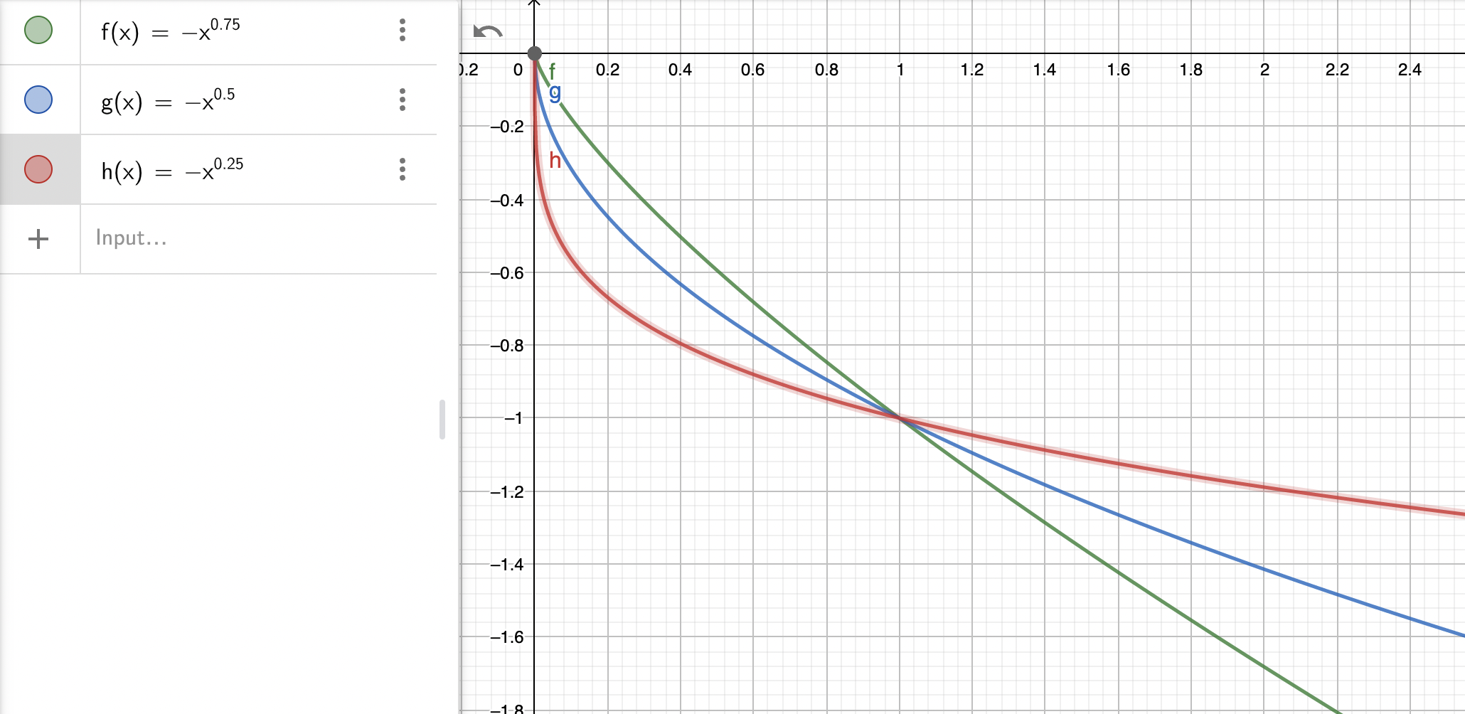
Cash gamma (green for $\alpha$=0.75, blue for 0.5 and red for 0.25)

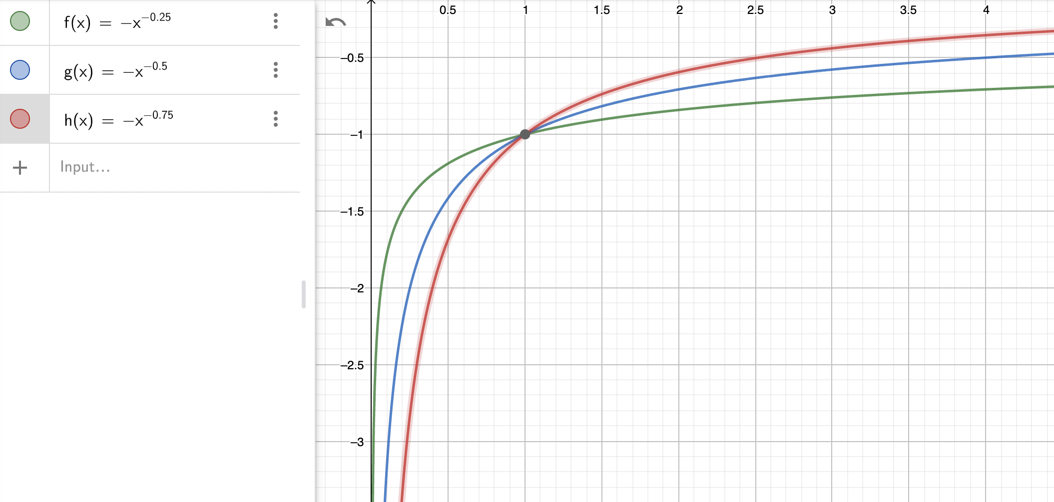
Cash strike density (green for $\alpha$=0.75, blue for 0.5 and red for 0.25)

---

Whilst reasonable care has been taken to verify the above formulas they may still contain errors. Please do not use them without independent verification.